4. Bayesian Neural Network

The idea is that, instead of learning specific weight (and bias) values in the neural network, the Bayesian approach learns weight distributions - from which we can sample to produce an output for a given input - to encode weight uncertainty. By training such NN, our aim is to learn approximative posterior distribution for each weight in NN. Thus, the number of parameters become double as compared to their non-bayesian counterparts because now every weight is represented by distribution parameters (mean and std if we consider distribution to be normal)

import numpy as np
import random
import tensorflow as tf
import matplotlib.pyplot as plt

from ai4water.utils.utils import get_version_info
from ai4water.utils.utils import TrainTestSplit
from ai4water.postprocessing import ProcessPredictions

from easy_mpl import plot

from utils import SAVE
from utils import set_rcParams
from utils import print_metrics
from utils import residual_plot, regression_plot
from utils import  make_data, BayesianNN
from utils import maybe_save_prediction

seed = 313
np.random.seed(seed)
random.seed(seed)
tf.random.set_seed(seed)

for lib, ver in get_version_info().items():
    print(lib, ver)

python 3.9.19 (main, Jun 18 2024, 09:35:09)
[GCC 11.4.0]
os posix
ai4water 1.07
lightgbm 4.4.0
xgboost 1.6.2
easy_mpl 0.21.4
SeqMetrics 1.3.4
tensorflow 2.10.1
keras.api._v2.keras 2.10.0
numpy 1.23.5
pandas 1.5.3
matplotlib 3.7.0
h5py 3.1.0
sklearn 1.0.2
optuna 3.6.1
skopt 0.9.0
seaborn 0.12.1

set_rcParams()

data, _, encoders= make_data(encoding='le')
X_train, X_test, y_train, y_test = TrainTestSplit(seed=142).\
    random_split_by_groups(x=data.iloc[:,0:-1], y=data.iloc[:, -1],
    groups=data['Adsorbent'])

print(X_train.shape, X_test.shape, y_train.shape, y_test.shape)

(2109, 17) (823, 17) (2109,) (823,)

input_features = X_train.columns.tolist()

hyperparameters

hidden_units = [8, 8]
learning_rate = 0.0017634228652070641
batch_size = 40
activation = "relu"
num_epochs = 500
alpha = 0.05

model building

model = BayesianNN(
    model = {"layers": dict(
        hidden_units=hidden_units,
        train_size =len(y_train),
        activation=activation,
        uncertainty_type='epistemic'
    )},
    category="DL",
    lr=learning_rate,
    batch_size=batch_size,
    epochs=num_epochs,
    input_features=input_features,
    #prefix="/mnt/datawaha/hyex/atr/playground/results/abcabc/"
)

            building DL model for
            regression problem using layers
Model: "model"
_________________________________________________________________
 Layer (type)                Output Shape              Param #
=================================================================
 Inputs (InputLayer)         [(None, 17)]              0

 batch_normalization (BatchN  (None, 17)               68
 ormalization)

 dense_variational (DenseVar  (None, 8)                10584
 iational)

 dense_variational_1 (DenseV  (None, 8)                2700
 ariational)

 dense (Dense)               (None, 1)                 9

=================================================================
Total params: 13,361
Trainable params: 13,327
Non-trainable params: 34
_________________________________________________________________
dot plot of model could not be plotted due to You must install pydot (`pip install pydot`) and install graphviz (see instructions at https://graphviz.gitlab.io/download/) for plot_model to work.

model training

model.update_weights('../models/BayesNN/weights.hdf5')

# model.fit(X_train, y_train, validation_data=(X_test, y_test),
#           verbose=0)

********** Successfully loaded weights from weights.hdf5 file **********

training data results

tr_predicted = []
for i in range(100):
    tr_predicted.append(model.predict(X_train, verbose=0))

tr_predicted = np.concatenate(tr_predicted, axis=1)

tr_std = np.std(tr_predicted, axis=1)
tr_mean = np.mean(tr_predicted, axis=1)

print_metrics(y_train, tr_mean, 'Train')

Train R2: 0.7226610545822302
Train R2 Score: 0.7160526716169855
Train RMSE Score: 37.7286517790873
Train MAE: 22.482232060089483

plot(tr_mean, '.', label="Prediction Mean", show=False)
plot(y_train.values, '.', label="True", ax_kws=dict(logy=True))

<Axes: >

test data results

test_predicted = []
for i in range(100):
    test_predicted.append(model.predict(X_test, verbose=0))

test_predicted = np.concatenate(test_predicted, axis=1)
test_mean = np.mean(test_predicted, axis=1)

f, ax = plt.subplots()
for i in range(50):

    plot(test_predicted[i], ax=ax, show=False,
         color='lightgray', alpha=0.7)

plot(test_mean[0:100], label="Mean Prediction", color="g", lw=2.0, ax=ax)
plt.show()

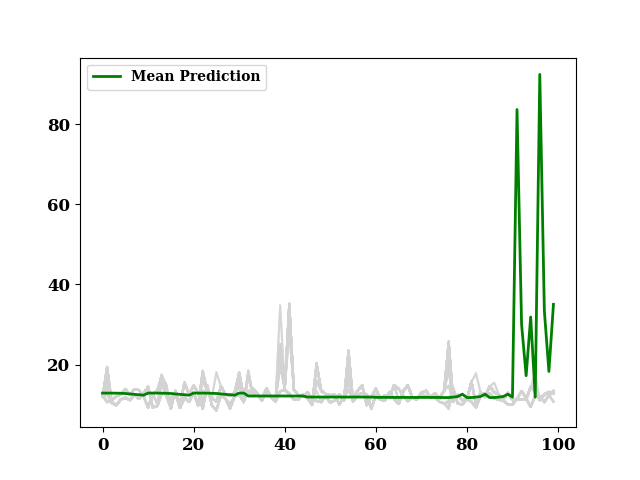
print_metrics(y_test, test_mean, 'Test')

Test R2: 0.7209191815981121
Test R2 Score: 0.7174685507293389
Test RMSE Score: 35.63016776422767
Test MAE: 22.460517638245157

maybe_save_prediction(y_train.values, tr_mean, 'bayes_train')

maybe_save_prediction(y_test.values, test_mean, 'bayes_test')

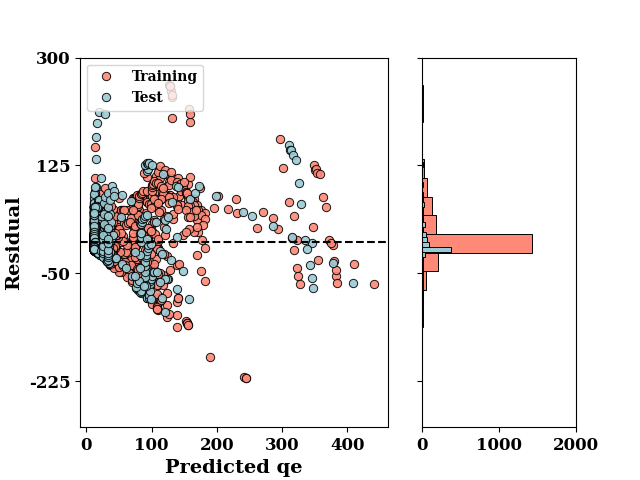
ax = residual_plot(y_train, tr_mean, y_test, test_mean, label="qe")
ax[0].set_ylim(-300, ax[0].get_ylim()[1])
if SAVE:
    plt.savefig("../manuscript/figures/residue_bayes",
                dpi=600, bbox_inches="tight")
plt.show()

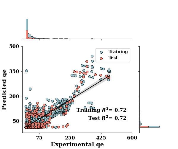
ax = regression_plot(y_train, tr_mean, y_test, test_mean)
ax.set_xlim(-20, ax.get_xlim()[1])
ax.set_ylim(-20, ax.get_ylim()[1])
if SAVE:
    plt.savefig("../manuscript/figures/reg_bayes", dpi=600, bbox_inches="tight")
plt.show()

lower = np.min(test_predicted[0:400], axis=1)
upper = np.max(test_predicted[0:400], axis=1)
_, ax = plt.subplots(figsize=(6, 3))
ax.fill_between(np.arange(len(lower)), upper, lower, alpha=0.5, color='C1')
p1 = ax.plot(test_mean[0:400], color="C1", label="Prediction")
p2 = ax.fill(np.NaN, np.NaN, color="C1", alpha=0.5)
plt.show()

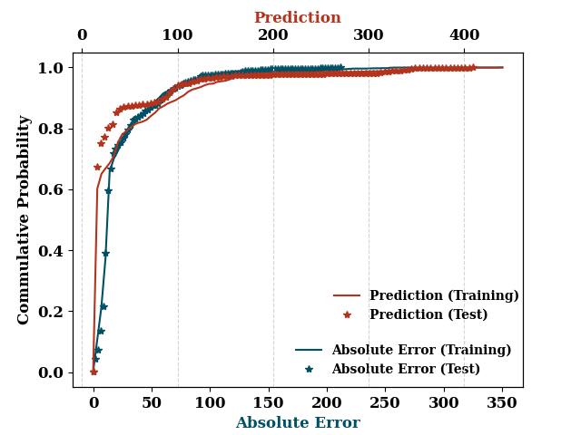
pp = ProcessPredictions('regression', 1, show=False)
output = pp.edf_plot(y_train, tr_mean,
                     label=("Absolute Error (Training)", "Prediction (Training)"))
output[1].legend(loc=(0.5, 0.18), frameon=False)
output = pp.edf_plot(y_test, test_mean, marker='*', ax=output[0], pred_axes=output[1],
                     label=("Absolute Error (Test)", "Prediction (Test)"))
output[1].legend(loc=(0.57, 0.18), frameon=False)
output[0].set_xlabel('Absolute Error', fontsize=12)
output[1].set_xlabel('Prediction', fontsize=12)
output[0].set_ylabel('Commulative Probability', fontsize=12)
if SAVE:
    plt.savefig("../manuscript/figures/bayes_edf", dpi=600, bbox_inches="tight")
plt.show()